Using SAS in Jupyter Lab
I'm sorry, but I need the text that you would like me to translate into naturalistic English.
Installing saspy
Launch python and use the following command to find the location of the saspy configuration file:
For example, if it returns:
<module 'saspy' from '
/home/ubuntu/miniconda3/envs/py39/lib/python3.9/site-packages/saspy/__init__.py'>
Open the directory /home/ubuntu/miniconda3/envs/py39/lib/python3.9/site-packages/saspy using SFTP and edit the sascfg.py file in that directory:

Change the saspath in the default section to the SAS installation location on your server. You can obtain this installation location in the Linux Shell using the following command:
which sas does not return anything
Reason
- The SAS application has not been added to the
PATHenvironment variable. - SAS is not installed on this server.
Solution
Please contact the administrator to install SAS and create a symbolic link to the executable in /usr/bin.
CFID users can simply use this path: /usr/local/SASHome/SASFoundation/9.4/bin/sas_u8.
Using SAS in Python
The official saspy reference code provided by SAS can be found at: saspy-examples
After trying it out, the recommended workflow is as follows.
Initialization
To use SAS data, you first need to specify the corresponding directory as a library in SAS. The following example specifies the directory /data/dataset/Compustat/d_global as a library in SAS and names it db.
import saspy

sas = saspy.SASsession()
ll = sas.submit('libname db "/data/dataset/Compustat/d_global";')
Reading Data
In this case, we assume that the core of data processing is done using Pandas. Therefore, the goal is to read SAS data into a Pandas DataFrame as efficiently as possible. If you need to convert it to another data type, you can do so from the Pandas DataFrame or explore other solutions.
Reading the entire table:

Efficiency
It is not recommended to use this method when reading large tables. Please refer to the next section.
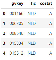
Reading selectively:
df = sas.sd2df(
    libref='db',
    table='g_names',
    dsopts={
        'where': 'costat = "A" and fic = "NLD"',
        'keep': ['gvkey', 'costat', 'fic'],
        # 'drop': ['conm', 'sedol'],
        'obs': 10
    }
)
df.head()

Handling
It is recommended to use the where and obs options. First, select a small amount of data based on certain conditions for observation, and then read the entire table after writing the processing code.
Once the data has been processed to a reasonable size, it can be stored as a Parquet file format for quick access to query results.
Try not to overwrite the variables directly returned by SAS (e.g., df in the example above) when reading large tables. Otherwise, it would be time-consuming to re-read the data every time there is a problem. Reading a 90GB SAS dataset takes about 10 minutes.
For more options, please refer to the documentation and sample code.
Advanced Queries
Select all data that matches the elements in a list:
df = sas.sd2df(
    libref='db',
    table='g_names',
    dsopts={
        'where': f'gvkey IN ({",".join([str(int(i)) for i gvkeys])})',
    }
)
df.head()
Query by date in the WHERE statement: